
Quadratic Integrate-and-Fire Model Crack Keygen For (LifeTime) Free [Mac/Win]
- durchsyspvantsatzt
- May 12, 2022
- 4 min read
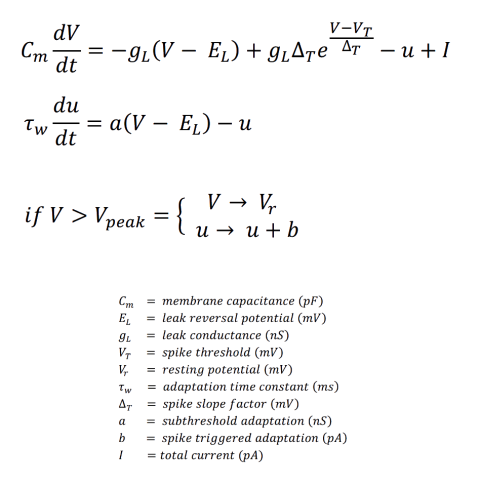
Quadratic Integrate-and-Fire Model Crack + Free PC/Windows [Latest] 2022 The Quadratic Integrate-and-Fire model offers a simple way of describing the dynamics of the neurons in your brain. It is basically a differential equation for the membrane potential of a neuron. The first thing you need to know about the Quadratic Integrate-and-Fire Model is that it models the dynamics of a cell in an extremely simplified manner. And you could, for example, expect it to work if the neuron is a single electrical compartment. But it can also be used to describe the dynamics of a network of neurons. We start with the intracellular dynamics of an integrate-and-fire neuron. And we will, of course, limit ourselves to the dynamics of a single cell. And we will model the neuron as a single compartment. The membrane potential V of a single compartment, let's call it the cell, evolves over time as a function of the input I. And it is given by the following equation. The time constant of the cell tau_c, is determined by the capacitance of the cell, by the permeability of the cell to K_+ ions, and by the surface area of the cell. And the threshold voltage is determined by the gate voltage of the cell. And so this is the equation of the single compartment of the cell. And the input to the cell is I, and it is a function of the voltage of the cell V. And so you are typically given a stimulus as a function of the membrane potential of the cell. And the input to the cell is I, and it is a function of the voltage of the cell V. And so we are now ready to define the dynamics of the entire network. And so the dynamics of the entire network is given by the following equation. Where K_+, is the permeability of the K+ ions, and so this is a constant for a single neuron. And n is a set of synapses, and it is a set of connections. And so the set of synapses is either excitatory or inhibitory. And they are connected to one another through one synapse and this synapse, we can call it P, is given by this equation. And so all these networks, and the set of synapses is either excitatory or inhibitory. And they are connected to one another through one synapse and this synapse, we can call it P, is given by this equation Quadratic Integrate-and-Fire Model Crack + Keygen For (LifeTime) Free The Python Simple Neuron Model The following example is used to illustrate how the `pyquadif` model can be integrated using the `pyquadif` Python module: ```python import pyquadif # Create a pyquadif model pyquadif.setup() # Generate an example neural network for i in range(3): # Create a neuron with threshold U = 0. # The activation of the neuron is the reset potential, # i.e., the membrane potential is 0 after it is reset. neuron = pyquadif.SimpleNeuron(0) # Connect the neuron to a summing node that # sums its inputs. neuron.connect(pyquadif.SummingNode()) # Connect the summing node to a relay node that # passes its input to the relay node. sumnode = pyquadif.SummingNode() sumnode.connect(relaynode) relaynode.connect(neuron) # Set up the integrate-and-fire circuit quads = pyquadif.RelayNode() quads.set(0, 0.1) quads.set(1, 0.2) quads.set(2, 0.3) # Add the relays to the circuit # Connect the input to the first relay quads.connect(input) # Connect the relay output to the input of the second relay quads.connect(quads.first_relay) # Connect the relay output of the second relay to the input of the third relay quads.connect(quads.second_relay) # Connect the output of the third relay to the input of the neuron quads.connect(neuron) # Set the threshold to U = 2 quads.set(neuron, 2) # Simulate the circuit pyquadif.run(quads) # Plot the membrane potential fig = plt.figure() ax 8e68912320 Quadratic Integrate-and-Fire Model (LifeTime) Activation Code [p] = [0]*(1-q*([1]-[1]*p)) + [1]*q*([1]-[1]*p)*[1] + p*(1-[1]*[1]) + [1]*[1]*([1]-[1]*p)*[1] [1] = [0]*(1-q*([1]-[1]*p)) + [1]*q*([1]-[1]*p)*[1] [1] = 1 [1] = 0 p = [-1]^n*[1] [1] = 0 #[1] = (1-q)*[1] + q [1] = 1 #q = 1/[2] n = 1 #Q = 1 n = 0 q = 1 #r = 0 r = 1 #q = 1/[2] [1] = (1-q)*[1] + q [1] = (1-[2]*[1])*[1] + [2]*[1] [1] = 0.5 If you don't want the oscillation to stop, you can make it a self-sustaining oscillator by adding a 0th order current term, because the term [1]-[1]*p works as a 0th order current. This enables the output value to keep increasing to infinity in some cases. import numpy as np import scipy as sp from scipy.integrate import quad import matplotlib.pyplot as plt from quadratic_integrate_and_fire import IAF class Circuit(IAF): def __init__(self): super().__init__(self.res, self.nstep, self.spd, self.diff, self.i_init, self.v_init, self.gate_cap, self.zero_cap, self.prec_corr, self.corr_int) self.bias = 0.01 self.charge = 0.000001 def init_param(self What's New in the? System Requirements For Quadratic Integrate-and-Fire Model: Windows 7 or higher 1.5 GB minimum of space iPad 2/3 or newer OS 4.3.3+ NVIDIA SHIELD Tablet or newer (SHIELD Tablet WiFi) Stick to the good old version number, don’t be afraid to go back to a stable version every now and then. Google Chrome OS (Chrome and Chrome for Android only at this time) Download Do note that Chrome Unpacked is built with the same toolset as Chrome OS and as such, you need
Related links:
Comments